AI PROMPT

Generative AI : Prompt Engineering

รูปแบบการแข่งขัน

การแข่งขันจะมีโจทย์ 3 รูปแบบ โดยการให้คะแนนและเรียงลำดับคะแนนจะทำไปเรื่อย ๆ จนกว่าจะหมดเวลา โดยมีรายละเอียดดังนี้:

การสร้างรูปภาพ:
- ใช้ generative AI สร้างรูปภาพให้เหมือนกับภาพที่กำหนด
- ตัวอย่างและการตัดสินความเหมือนของรูปภาพ: ลิงก์ตัวอย่าง
การเขียนโปรแกรม:
- เขียนโปรแกรมให้ทำงานตามจุดประสงค์ที่กำหนด หรือแก้ไขโปรแกรมที่มีความผิดพลาด
- ใช้ภาษา Python และทำงานบน Colab เป็นหลัก
การสร้าง AI:
- ใช้ generative AI สร้าง AI จากข้อมูลชุดฝึกสอนเพื่อทำนายข้อมูลชุดทดสอบ
- ตัวอย่างข้อมูล โมเดล และการวัดประสิทธิภาพ: ลิงก์ตัวอย่าง 1, ลิงก์ตัวอย่าง 2

การให้คะแนน:

รูปแบบที่ 1: ความเหมือนของภาพที่สร้างขึ้นกับภาพต้นฉบับ
รูปแบบที่ 2: ความถูกต้องของโปรแกรม, ประสิทธิภาพในการแก้ปัญหา
รูปแบบที่ 3: ความแม่นยำของโมเดล AI ที่สร้างขึ้น

ผู้เข้าแข่งขันต้องส่ง prompt ในทุกโจทย์ปัญหาของการแข่งขัน

เงื่อนไขการแข่งขัน:

ใช้ generative AI เวอร์ชั่นใดก็ได้ไม่มีข้อจำกัด
ใช้คอมพิวเตอร์ของวิทยาลัยที่มีอินเตอร์เน็ต
นำอุปกรณ์เข้าห้องแข่งขันได้ไม่จำกัด
ปรึกษากันในทีมเท่านั้น ไม่อนุญาตให้สอบถามบุคคลอื่น

ข้อแนะนำในการแข่งขัน:

สมัครสมาชิก Colab ล่วงหน้า
สมัครสมาชิก Kaggle ล่วงหน้า

Generative AI : Prompt Engineering

1.1 เว็บไซต์สร้างภาพด้วย Ai

1.2 ตารางประเภท Prompt

1.3 เว็บไซต์นำเสนอ Prompt

1.4 การเปรียบเทียบความเหมือนของภาพ

2.1 การเรียนรู้แบบมีผู้สอน

2.2 ไลบรารี scikit-learn

2.3 อธิบายโค้ด Classifier comparison

2.4 โค้ดจำแนก iris ใน Kaggle

2.5 โค้ดจำแนก iris ใน colab

2.6 Prompt ที่ใช้

3.1 โจทย์เขียนโปรแกรม

*ส่งคำตอบการสร้างภาพ

*ส่งคำตอบการเขียนโปรแกรม

*ส่งคำตอบการเทรนโมเดล Ai

1.1 เว็บไซต์สร้างภาพด้วย Ai

1.2 ตารางประเภท Prompt

Table of Styles and Types

Style	Description	Examples
Realistic	Detailed and lifelike, resembling a photograph.	A realistic landscape at sunset, a photorealistic portrait of a person
Cartoon	Simplified and exaggerated, often with bold colors and outlines.	A cartoon dog riding a skateboard, a superhero with cartoonish proportions
Fantasy	Elements of magic and mythical creatures, often with vibrant and otherworldly visuals.	A dragon flying over a mystical forest, a wizard casting a spell in a fantasy world
Abstract	Focused on shapes, colors, and patterns rather than realistic depictions.	An abstract representation of emotion, a colorful geometric pattern
Watercolor	Soft and fluid, mimicking the look of a watercolor painting.	A watercolor landscape of mountains, a watercolor portrait with delicate brush strokes
Cyberpunk	Futuristic and dystopian, with neon lights and a high-tech aesthetic.	A cyberpunk cityscape at night, a character with cybernetic enhancements
Vintage	Aged and nostalgic, often with a sepia tone or muted colors.	A vintage car in a retro setting, a 1950s-style diner with classic decor
Surreal	Dreamlike and bizarre, blending reality with the fantastical.	A melting clock in a desert, a floating island with impossible architecture
Minimalist	Clean and simple, focusing on a few key elements or shapes.	A minimalist landscape with a single tree, a portrait with a few bold lines
Steampunk	Inspired by the Victorian era and industrial machinery, with gears and steam-powered devices.	A steampunk airship in a cloudy sky, a character wearing steampunk goggles and attire
Pixel Art	Digital art created with pixels, resembling old video games or computer graphics.	A pixel art city with tiny buildings, a pixelated character in a forest
Noir	Dark and moody, with high contrast and shadowy scenes.	A noir detective in a dimly lit office, a mysterious figure in a rain-soaked alleyway
Impressionist	Inspired by the Impressionist art movement, with visible brush strokes and a focus on light and color.	An impressionist painting of a bustling café, a landscape with dappled sunlight
Pop Art	Bold and colorful, often using comic book-style elements and popular culture references.	A pop art portrait of a celebrity, a cityscape with bright, contrasting colors
Retro Futuristic	A blend of past and future styles, often with elements of 1950s or 1980s visions of the future.	A retro-futuristic robot with chrome and neon accents, a city with flying cars and retro architecture
Gothic	Dark and eerie, with elements of horror and the macabre.	A gothic castle under a stormy sky, a vampire in a shadowy room

1.3 เว็บไซต์นำเสนอ Prompt

1.4 การเปรียบเทียบความเหมือนของภาพ

2.1 การเรียนรู้แบบมีผู้สอน

2.2 ไลบรารี scikit-learn

จาก ลิงก์อ้างอิง

scikit-learn คือไลบรารีในภาษา Python ที่ใช้สำหรับการเรียนรู้ของเครื่อง (Machine Learning) โดยเฉพาะ มันมีเครื่องมือและฟังก์ชันที่ช่วยในการสร้าง ทดสอบ และใช้งานโมเดล Machine Learning ได้อย่างง่ายดาย รวมถึงการประมวลผลข้อมูล การจำแนกประเภท การถดถอย (Regression) การจัดกลุ่มข้อมูล (Clustering) และอื่นๆ อีกมากมาย
scikit-learn ถูกออกแบบให้ใช้งานง่าย เหมาะสำหรับทั้งผู้เริ่มต้นและผู้ที่มีประสบการณ์ นอกจากนี้ยังมีการบูรณาการกับไลบรารีอื่นๆ ของ Python เช่น NumPy และ pandas ซึ่งทำให้การประมวลผลและวิเคราะห์ข้อมูลทำได้อย่างมีประสิทธิภาพ

การเปรียบเทียบตัวจำแนกประเภทข้อมูล (Classifier) ใน scikit-learn เป็นการวิเคราะห์ความสามารถของโมเดลต่างๆ ในการแยกประเภทข้อมูล เช่น การทำนายว่าข้อมูลอยู่ในกลุ่มใด เช่น ใช่/ไม่ใช่, ดี/ไม่ดี หรือประเภทอื่นๆ

scikit-learn มีเครื่องมือสำหรับสร้างและเปรียบเทียบตัวจำแนกประเภทมากมาย เช่น:

ในกระบวนการเปรียบเทียบ โมเดลเหล่านี้จะถูกทดสอบกับข้อมูลเดียวกัน เพื่อดูว่าโมเดลไหนทำงานได้ดีที่สุดในสถานการณ์ที่กำหนด ผลลัพธ์อาจขึ้นอยู่กับคุณภาพของข้อมูล การปรับแต่งพารามิเตอร์ และความเหมาะสมของโมเดลกับงานนั้นๆ

2.3 อธิบายโค้ด Classifier comparison

จาก ลิงก์อ้างอิง
โค้ดนี้เป็นส่วนหนึ่งของโปรเจกต์ที่เกี่ยวข้องกับการแสดงผล Decision Boundaries ของโมเดล Machine Learning โดยใช้หลายประเภทของตัวจำแนก (classifier) ในการสร้างและวิเคราะห์ข้อมูลที่มีการแจกแจงข้อมูลที่ต่างกัน ต่อไปนี้เป็นการอธิบายแต่ละบรรทัดในโค้ดอย่างละเอียด:

ส่วนที่ 1: การนำเข้าไลบรารีและโมดูลต่าง ๆ

import matplotlib.pyplot as plt
import numpy as np
from matplotlib.colors import ListedColormap

matplotlib.pyplot as plt: ใช้สำหรับการสร้างกราฟและการแสดงผลข้อมูลแบบ 2D ใน Python
numpy as np: ใช้สำหรับการจัดการกับข้อมูลในรูปแบบอาร์เรย์, การคำนวณทางคณิตศาสตร์ที่ต้องการความรวดเร็ว
ListedColormap จาก matplotlib.colors: ใช้สำหรับการสร้างสีที่ระบุเองสำหรับการแสดงผลข้อมูล

ส่วนที่ 2: การนำเข้าชุดข้อมูลและโมเดล Machine Learning

from sklearn.datasets import make_circles, make_classification, make_moons

make_circles: สร้างชุดข้อมูลที่มีการแจกแจงเป็นวงกลมสองชั้น
make_classification: สร้างชุดข้อมูลที่ใช้สำหรับการทดสอบและเทรนโมเดลการจัดประเภท (classification)
make_moons: สร้างชุดข้อมูลที่มีรูปแบบคล้ายเสี้ยวพระจันทร์สองเสี้ยว

from sklearn.discriminant_analysis import QuadraticDiscriminantAnalysis
from sklearn.ensemble import AdaBoostClassifier, RandomForestClassifier
from sklearn.gaussian_process import GaussianProcessClassifier
from sklearn.gaussian_process.kernels import RBF
from sklearn.inspection import DecisionBoundaryDisplay
from sklearn.model_selection import train_test_split
from sklearn.naive_bayes import GaussianNB
from sklearn.neighbors import KNeighborsClassifier
from sklearn.neural_network import MLPClassifier
from sklearn.pipeline import make_pipeline
from sklearn.preprocessing import StandardScaler
from sklearn.svm import SVC
from sklearn.tree import DecisionTreeClassifier

โมดูลเหล่านี้นำเข้าตัวจำแนก (classifier) หลายประเภท รวมถึงเครื่องมือและฟังก์ชันต่าง ๆ สำหรับการสร้างโมเดล, การปรับแต่งข้อมูล, และการแสดงผล decision boundary:

QuadraticDiscriminantAnalysis: ตัวจำแนกที่ใช้การวิเคราะห์การแยกแยะเชิงกำลังสอง (quadratic discriminant analysis)
AdaBoostClassifier: ตัวจำแนกที่ใช้เทคนิค AdaBoost สำหรับการเสริมกำลังการเรียนรู้
RandomForestClassifier: ตัวจำแนกที่ใช้เทคนิค Random Forest ซึ่งเป็นการรวมกันของหลาย decision trees
GaussianProcessClassifier: ตัวจำแนกที่ใช้กระบวนการ Gaussian ในการเรียนรู้
RBF: Kernel ที่ใช้ใน Gaussian Process
DecisionBoundaryDisplay: ใช้สำหรับการแสดง decision boundary ของโมเดล
train_test_split: แบ่งชุดข้อมูลออกเป็นชุดข้อมูลฝึกสอนและทดสอบ
GaussianNB: ตัวจำแนกแบบ Naive Bayes ที่อิงตามการแจกแจงแบบ Gaussian
KNeighborsClassifier: ตัวจำแนกที่ใช้วิธี k-nearest neighbors (k-NN)
MLPClassifier: ตัวจำแนกแบบ Neural Network ที่เรียกว่า Multi-layer Perceptron
make_pipeline: สร้าง pipeline สำหรับการทำ preprocessing ข้อมูลและการสร้างโมเดล
StandardScaler: ใช้สำหรับการทำให้ข้อมูลมีสเกลที่เป็นมาตรฐาน
SVC: ตัวจำแนกที่ใช้วิธี Support Vector Classifier
DecisionTreeClassifier: ตัวจำแนกที่ใช้เทคนิค Decision Tree

ส่วนที่ 3: นิยามตัวจำแนก

names = [
    "Nearest Neighbors",
    "Linear SVM",
    "RBF SVM",
    "Gaussian Process",
    "Decision Tree",
    "Random Forest",
    "Neural Net",
    "AdaBoost",
    "Naive Bayes",
    "QDA",
]

names: เป็นรายการของชื่อที่ใช้เรียกตัวจำแนกแต่ละตัว ซึ่งจะใช้ในการแสดงผลหรือการอ้างอิงในภายหลัง ชื่อเหล่านี้อธิบายถึงโมเดลต่าง ๆ ที่อยู่ในรายการ classifiers

classifiers = [
    KNeighborsClassifier(3),
    SVC(kernel="linear", C=0.025, random_state=42),
    SVC(gamma=2, C=1, random_state=42),
    GaussianProcessClassifier(1.0 * RBF(1.0), random_state=42),
    DecisionTreeClassifier(max_depth=5, random_state=42),
    RandomForestClassifier(
        max_depth=5, n_estimators=10, max_features=1, random_state=42
    ),
    MLPClassifier(alpha=1, max_iter=1000, random_state=42),
    AdaBoostClassifier(algorithm="SAMME", random_state=42),
    GaussianNB(),
    QuadraticDiscriminantAnalysis(),
]

ส่วนที่ 4: สร้างชุดข้อมูล `X` และ `y`

X, y = make_classification(
    n_features=2, n_redundant=0, n_informative=2, random_state=1, n_clusters_per_class=1
)

make_classification: ฟังก์ชันนี้ใช้สร้างชุดข้อมูลจำลองที่สามารถนำมาใช้ในการจำแนกประเภท (classification) โดยกำหนดพารามิเตอร์ดังนี้:
- n_features=2: สร้างคุณลักษณะ (features) 2 ตัว
- n_redundant=0: ไม่มีคุณลักษณะที่ซ้ำซ้อน
- n_informative=2: คุณลักษณะที่มีประโยชน์ต่อการจำแนกประเภทมี 2 ตัว
- random_state=1: ใช้สำหรับกำหนดค่าเริ่มต้นของตัวเลขสุ่ม เพื่อให้สามารถทำซ้ำผลลัพธ์ได้
- n_clusters_per_class=1: กำหนดให้แต่ละคลาสมีหนึ่งกลุ่ม (cluster) ของข้อมูล

ผลลัพธ์คือชุดข้อมูล X (คุณลักษณะ) และ y (ป้ายกำกับหรือคลาส) ที่ใช้ในการจำแนก

เพิ่มความไม่เป็นเชิงเส้นในข้อมูล `X`

rng = np.random.RandomState(2)
X += 2 * rng.uniform(size=X.shape)

rng = np.random.RandomState(2): สร้างตัวสุ่มที่ใช้สำหรับการสร้างตัวเลขสุ่ม โดยกำหนดค่า seed เป็น 2 เพื่อให้การทำซ้ำผลลัพธ์เป็นไปได้
X += 2 * rng.uniform(size=X.shape): เพิ่มค่าสุ่มที่สร้างขึ้นจากการแจกแจงแบบสม่ำเสมอ (uniform distribution) เข้าไปในข้อมูล X เพื่อทำให้ข้อมูลมีความซับซ้อนและไม่เป็นเชิงเส้นมากขึ้น

เก็บชุดข้อมูลไว้ในตัวแปร `linearly_separable`

linearly_separable = (X, y)

linearly_separable: เก็บคู่ของข้อมูล X และ y ที่สร้างขึ้นมาในรูปของทูเพิล (tuple) เพื่อใช้ในภายหลัง

สร้างชุดข้อมูลอื่น ๆ และจัดเก็บใน `datasets`

datasets = [
    make_moons(noise=0.3, random_state=0),
    make_circles(noise=0.2, factor=0.5, random_state=1),
    linearly_separable,
]

make_moons(noise=0.3, random_state=0): สร้างชุดข้อมูลที่มีรูปร่างเป็นเสี้ยวพระจันทร์สองเสี้ยว โดยมีการเพิ่ม noise (ความไม่สมบูรณ์ของข้อมูล) เข้าไปเล็กน้อย (noise=0.3) และกำหนด random_state=0 เพื่อให้ทำซ้ำได้
make_circles(noise=0.2, factor=0.5, random_state=1): สร้างชุดข้อมูลที่มีการกระจายตัวเป็นวงกลมสองชั้น โดยมี noise (noise=0.2) และกำหนด factor=0.5 เพื่อระบุขนาดของวงกลมที่เล็กลง และกำหนด random_state=1 เพื่อให้ทำซ้ำได้
linearly_separable: ชุดข้อมูลที่สร้างขึ้นมาในขั้นตอนก่อนหน้านี้ซึ่งมีการแจกแจงแบบเชิงเส้น

บทสรุป

โค้ดนี้สร้างชุดข้อมูลจำลองสามชุดที่มีลักษณะการแจกแจงแตกต่างกัน เพื่อใช้ในการทดสอบตัวจำแนกที่กำหนดไว้ก่อนหน้านี้:

make_moons: ชุดข้อมูลที่มีรูปร่างเป็นเสี้ยวพระจันทร์
make_circles: ชุดข้อมูลที่มีรูปร่างเป็นวงกลมสองชั้น
linearly_separable: ชุดข้อมูลที่สร้างขึ้นให้สามารถแยกได้ด้วยเส้นตรงแต่มีการเพิ่มความไม่เป็นเชิงเส้นเข้าไป

ส่วนที่ 5: การแสดงผลชุดข้อมูลและผลลัพธ์จากการจำแนก

โค้ดนี้ทำการแสดงผลชุดข้อมูลและผลลัพธ์จากตัวจำแนก (classifiers) ที่ถูกเทรนบนชุดข้อมูลนั้น โดยแสดงเป็นกริด (grid) ที่มีหลายแถวและหลายคอลัมน์ แต่ละแถวแสดงข้อมูลและการจำแนกของชุดข้อมูลหนึ่ง ๆ และแต่ละคอลัมน์แสดงผลการจำแนกจากตัวจำแนกที่แตกต่างกัน ต่อไปนี้เป็นคำอธิบายโดยละเอียดของโค้ด:

การสร้างฟิกเกอร์และการเตรียมตัวแปร

figure = plt.figure(figsize=(27, 9))
i = 1

figure = plt.figure(figsize=(27, 9)): สร้างฟิกเกอร์ (figure) ขนาดใหญ่ (27×9 นิ้ว) ที่จะใช้ในการวาดกราฟ
i = 1: กำหนดตัวแปร i เพื่อใช้ในการติดตามตำแหน่งของ subplot ในกริด

การวนลูปชุดข้อมูล (`datasets`)

for ds_cnt, ds in enumerate(datasets):
    # preprocess dataset, split into training and test part
    X, y = ds
    X_train, X_test, y_train, y_test = train_test_split(
        X, y, test_size=0.4, random_state=42
    )

for ds_cnt, ds in enumerate(datasets):: วนลูปผ่านชุดข้อมูลแต่ละชุดใน datasets
X, y = ds: แยกข้อมูล X (คุณลักษณะ) และ y (ป้ายกำกับหรือคลาส) ออกจากทูเพิล ds
train_test_split(...): แบ่งข้อมูล X และ y ออกเป็นชุดข้อมูลฝึกสอน (X_train, y_train) และทดสอบ (X_test, y_test) โดยใช้สัดส่วน 60:40 (test_size=0.4)

การกำหนดขอบเขตของกราฟ

    x_min, x_max = X[:, 0].min() - 0.5, X[:, 0].max() + 0.5
    y_min, y_max = X[:, 1].min() - 0.5, X[:, 1].max() + 0.5

x_min, x_max, y_min, y_max: กำหนดขอบเขตของแกน x และ y โดยขยายขอบเขตออกไปเล็กน้อย (-0.5 และ +0.5) เพื่อให้การแสดงผลดูชัดเจนขึ้น

การแสดงผลชุดข้อมูลต้นฉบับ

    cm = plt.cm.RdBu
    cm_bright = ListedColormap(["#FF0000", "#0000FF"])
    ax = plt.subplot(len(datasets), len(classifiers) + 1, i)
    if ds_cnt == 0:
        ax.set_title("Input data")
    # Plot the training points
    ax.scatter(X_train[:, 0], X_train[:, 1], c=y_train, cmap=cm_bright, edgecolors="k")
    # Plot the testing points
    ax.scatter(
        X_test[:, 0], X_test[:, 1], c=y_test, cmap=cm_bright, alpha=0.6, edgecolors="k"
    )
    ax.set_xlim(x_min, x_max)
    ax.set_ylim(y_min, y_max)
    ax.set_xticks(())
    ax.set_yticks(())
    i += 1
    # iterate over classifiers
    for name, clf in zip(names, classifiers):
        ax = plt.subplot(len(datasets), len(classifiers) + 1, i)

        clf = make_pipeline(StandardScaler(), clf)
        clf.fit(X_train, y_train)
        score = clf.score(X_test, y_test)
        DecisionBoundaryDisplay.from_estimator(
            clf, X, cmap=cm, alpha=0.8, ax=ax, eps=0.5
        )
        # Plot the training points
        ax.scatter(
            X_train[:, 0], X_train[:, 1], c=y_train, cmap=cm_bright, edgecolors="k"
        )
        # Plot the testing points
        ax.scatter(
            X_test[:, 0],
            X_test[:, 1],
            c=y_test,
            cmap=cm_bright,
            edgecolors="k",
            alpha=0.6,
        )
        ax.set_xlim(x_min, x_max)
        ax.set_ylim(y_min, y_max)
        ax.set_xticks(())
        ax.set_yticks(())
        if ds_cnt == 0:
            ax.set_title(name)
        ax.text(
            x_max - 0.3,
            y_min + 0.3,
            ("%.2f" % score).lstrip("0"),
            size=15,
            horizontalalignment="right",
        )
        i += 1

cm = plt.cm.RdBu: กำหนด color map ที่จะใช้สำหรับการแสดงผล decision boundary
cm_bright = ListedColormap(["#FF0000", "#0000FF"]): กำหนด color map ที่ใช้แสดงผลข้อมูล (#FF0000 สีแดง, #0000FF สีน้ำเงิน)
ax = plt.subplot(...): สร้าง subplot ในตำแหน่งที่ i ของกริด มีขนาด len(datasets) แถว และ len(classifiers) + 1 คอลัมน์
if ds_cnt == 0:: ตั้งชื่อคอลัมน์แรกเป็น “Input data” ในแถวแรก
ax.scatter(...): แสดงผลจุดข้อมูล X_train และ X_test ลงใน subplot ด้วยสีตามป้ายกำกับ y_train และ y_test
ax.set_xlim(x_min, x_max): กำหนดขอบเขตของแกน x
ax.set_ylim(y_min, y_max): กำหนดขอบเขตของแกน y
ax.set_xticks(()), ax.set_yticks(()): ซ่อน tick marks บนแกน x และ y
i += 1: เพิ่มค่า i เพื่อเตรียมวาง subplot ถัดไป

2.4 โค้ดจำแนก iris ใน Kaggle

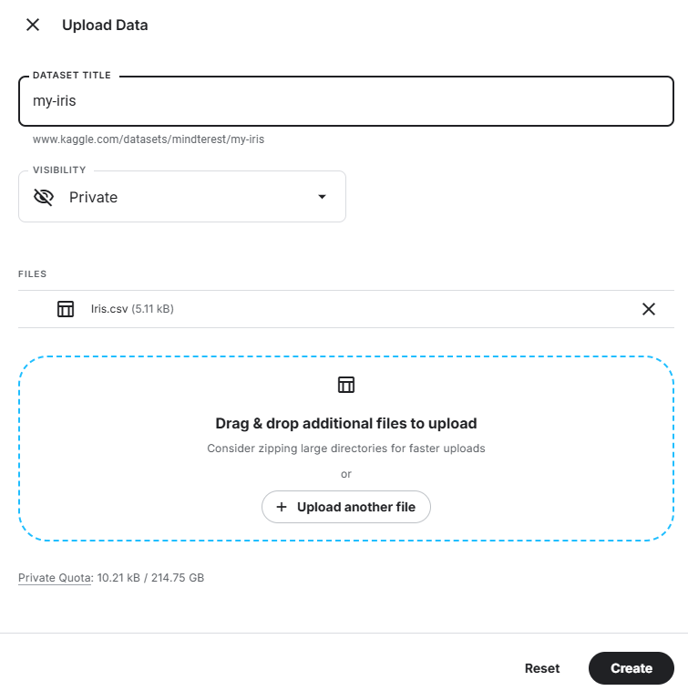
ก่อนอื่นต้องทำการอัปโหลด Dataset ก่อน

โค้ดที่ได้จากพร้อมพ์

ทำให้โค้ดต่อไปนนี้สามารถทำงานได้บน Kaggle

import matplotlib.pyplot as plt
import numpy as np
import pandas as pd
from matplotlib.colors import ListedColormap
from sklearn.discriminant_analysis import QuadraticDiscriminantAnalysis
from sklearn.ensemble import AdaBoostClassifier, RandomForestClassifier
from sklearn.gaussian_process import GaussianProcessClassifier
from sklearn.gaussian_process.kernels import RBF
from sklearn.inspection import DecisionBoundaryDisplay
from sklearn.model_selection import train_test_split
from sklearn.naive_bayes import GaussianNB
from sklearn.neighbors import KNeighborsClassifier
from sklearn.neural_network import MLPClassifier
from sklearn.pipeline import make_pipeline
from sklearn.preprocessing import StandardScaler
from sklearn.svm import SVC
from sklearn.tree import DecisionTreeClassifier

# Load the CSV file into a DataFrame
data = pd.read_csv('/kaggle/input/your-dataset-name/your-dataset.csv')
# แก้เป็น my-iris/Iris.csv
# Display the column names to understand the actual names in the CSV
print("Columns in the DataFrame:", data.columns)

# Adjust column names based on actual columns in your CSV
# For this example, we use the typical column names of the Iris dataset
X = data[['PetalLengthCm', 'PetalWidthCm']].values  # Use only the first two features for visualization
y = data['Species'].astype('category').cat.codes  # Convert species to numeric codes

# Define classifier names and classifiers
names = [
    "Nearest Neighbors",
    "Linear SVM",
    "RBF SVM",
    "Gaussian Process",
    "Decision Tree",
    "Random Forest",
    "Neural Net",
    "AdaBoost",
    "Naive Bayes",
    "QDA",
]

classifiers = [
    KNeighborsClassifier(3),
    SVC(kernel="linear", C=0.025, random_state=42),
    SVC(gamma=2, C=1, random_state=42),
    GaussianProcessClassifier(1.0 * RBF(1.0), random_state=42),
    DecisionTreeClassifier(max_depth=5, random_state=42),
    RandomForestClassifier(
        max_depth=5, n_estimators=10, max_features=1, random_state=42
    ),
    MLPClassifier(alpha=1, max_iter=1000, random_state=42),
    AdaBoostClassifier(algorithm="SAMME", random_state=42),
    GaussianNB(),
    QuadraticDiscriminantAnalysis(),
]

# Split dataset into training and test parts
X_train, X_test, y_train, y_test = train_test_split(
    X, y, test_size=0.4, random_state=42
)

# Define grid limits for the first two features
x_min, x_max = X[:, 0].min() - 0.5, X[:, 0].max() + 0.5
y_min, y_max = X[:, 1].min() - 0.5, X[:, 1].max() + 0.5

# Create figure
figure = plt.figure(figsize=(15, 3))
i = 1

# Plot the dataset
cm = plt.cm.RdBu
cm_bright = ListedColormap(["#FF0000", "#0000FF", "#00FF00"])
ax = plt.subplot(1, len(classifiers) + 1, i)
ax.set_title("Input data")

# Plot the training points
ax.scatter(X_train[:, 0], X_train[:, 1], c=y_train, cmap=cm_bright, edgecolors="k")
# Plot the testing points
ax.scatter(
    X_test[:, 0], X_test[:, 1], c=y_test, cmap=cm_bright, alpha=0.6, edgecolors="k"
)
ax.set_xlim(x_min, x_max)
ax.set_ylim(y_min, y_max)
ax.set_xticks(())
ax.set_yticks(())
i += 1

# Iterate over classifiers
for name, clf in zip(names, classifiers):
    ax = plt.subplot(1, len(classifiers) + 1, i)

    clf = make_pipeline(StandardScaler(), clf)
    clf.fit(X_train, y_train)
    score = clf.score(X_test, y_test)
    DecisionBoundaryDisplay.from_estimator(
        clf, X, cmap=cm, alpha=0.8, ax=ax, eps=0.5
    )

    # Plot the training points
    ax.scatter(
        X_train[:, 0], X_train[:, 1], c=y_train, cmap=cm_bright, edgecolors="k"
    )
    # Plot the testing points
    ax.scatter(
        X_test[:, 0],
        X_test[:, 1],
        c=y_test,
        cmap=cm_bright,
        edgecolors="k",
        alpha=0.6,
    )

    ax.set_xlim(x_min, x_max)
    ax.set_ylim(y_min, y_max)
    ax.set_xticks(())
    ax.set_yticks(())
    ax.set_title(name)
    ax.text(
        x_max - 0.3,
        y_min + 0.3,
        ("%.2f" % score).lstrip("0"),
        size=15,
        horizontalalignment="right",
    )
    i += 1

plt.tight_layout()
plt.show()

2.5 โค้ดจำแนก iris ใน colab

จากลิงก์ iris classification.ipynb

import matplotlib.pyplot as plt
import numpy as np
import pandas as pd
import io
from google.colab import files
from matplotlib.colors import ListedColormap
from sklearn.discriminant_analysis import QuadraticDiscriminantAnalysis
from sklearn.ensemble import AdaBoostClassifier, RandomForestClassifier
from sklearn.gaussian_process import GaussianProcessClassifier
from sklearn.gaussian_process.kernels import RBF
from sklearn.inspection import DecisionBoundaryDisplay
from sklearn.model_selection import train_test_split
from sklearn.naive_bayes import GaussianNB
from sklearn.neighbors import KNeighborsClassifier
from sklearn.neural_network import MLPClassifier
from sklearn.pipeline import make_pipeline
from sklearn.preprocessing import StandardScaler
from sklearn.svm import SVC
from sklearn.tree import DecisionTreeClassifier

# Upload file
uploaded = files.upload()

# Load the CSV file into a DataFrame
for filename in uploaded.keys():
    data = pd.read_csv(io.BytesIO(uploaded[filename]))

# Display the column names to understand the actual names in the CSV
print("Columns in the DataFrame:", data.columns)

# Adjust column names based on actual columns in your CSV
# For this example, we use the typical column names of the Iris dataset
X = data[['PetalLengthCm', 'PetalWidthCm']].values  # Use only the first two features for visualization
y = data['Species'].astype('category').cat.codes  # Convert species to numeric codes

# Define classifier names and classifiers
names = [
    "Nearest Neighbors",
    "Linear SVM",
    "RBF SVM",
    "Gaussian Process",
    "Decision Tree",
    "Random Forest",
    "Neural Net",
    "AdaBoost",
    "Naive Bayes",
    "QDA",
]

classifiers = [
    KNeighborsClassifier(3),
    SVC(kernel="linear", C=0.025, random_state=42),
    SVC(gamma=2, C=1, random_state=42),
    GaussianProcessClassifier(1.0 * RBF(1.0), random_state=42),
    DecisionTreeClassifier(max_depth=5, random_state=42),
    RandomForestClassifier(
        max_depth=5, n_estimators=10, max_features=1, random_state=42
    ),
    MLPClassifier(alpha=1, max_iter=1000, random_state=42),
    AdaBoostClassifier(algorithm="SAMME", random_state=42),
    GaussianNB(),
    QuadraticDiscriminantAnalysis(),
]

# Split dataset into training and test parts
X_train, X_test, y_train, y_test = train_test_split(
    X, y, test_size=0.4, random_state=42
)

# Define grid limits for the first two features
x_min, x_max = X[:, 0].min() - 0.5, X[:, 0].max() + 0.5
y_min, y_max = X[:, 1].min() - 0.5, X[:, 1].max() + 0.5

# Create figure
figure = plt.figure(figsize=(27, 3))
i = 1

# Plot the dataset
cm = plt.cm.RdBu
cm_bright = ListedColormap(["#FF0000", "#0000FF", "#00FF00"])
ax = plt.subplot(1, len(classifiers) + 1, i)
ax.set_title("Input data")

# Plot the training points
ax.scatter(X_train[:, 0], X_train[:, 1], c=y_train, cmap=cm_bright, edgecolors="k")
# Plot the testing points
ax.scatter(
    X_test[:, 0], X_test[:, 1], c=y_test, cmap=cm_bright, alpha=0.6, edgecolors="k"
)
ax.set_xlim(x_min, x_max)
ax.set_ylim(y_min, y_max)
ax.set_xticks(())
ax.set_yticks(())
i += 1

# Iterate over classifiers
for name, clf in zip(names, classifiers):
    ax = plt.subplot(1, len(classifiers) + 1, i)

    clf = make_pipeline(StandardScaler(), clf)
    clf.fit(X_train, y_train)
    score = clf.score(X_test, y_test)
    DecisionBoundaryDisplay.from_estimator(
        clf, X, cmap=cm, alpha=0.8, ax=ax, eps=0.5
    )

    # Plot the training points
    ax.scatter(
        X_train[:, 0], X_train[:, 1], c=y_train, cmap=cm_bright, edgecolors="k"
    )
    # Plot the testing points
    ax.scatter(
        X_test[:, 0],
        X_test[:, 1],
        c=y_test,
        cmap=cm_bright,
        edgecolors="k",
        alpha=0.6,
    )

    ax.set_xlim(x_min, x_max)
    ax.set_ylim(y_min, y_max)
    ax.set_xticks(())
    ax.set_yticks(())
    ax.set_title(name)
    ax.text(
        x_max - 0.3,
        y_min + 0.3,
        ("%.2f" % score).lstrip("0"),
        size=15,
        horizontalalignment="right",
    )
    i += 1

plt.tight_layout()
plt.show()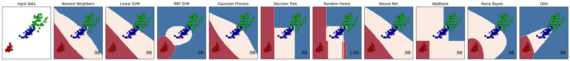

2.6 Prompt ที่ใช้

จงอธิบายโค้ดต่อไปนี้โดยละเอียด

ดัดแปลงโค้ดทั้งหมดข้างต้นเพื่อจำแนกข้อมูล iris.csv เพียงชุดข้อมูลเดียว

ดัดแปลงโค้ดให้ผู้ใช้อัพโหลดไฟล์ iris.csv เอง

ขอโค้ดจำแนก iris.csv ใหม่โดยสามารถอัพโหลดไฟล์ใน colab ได้

ปรับแก้โค้ดให้ใช้ข้อมูลจากทั้ง 4 คอลัมน์ SepalLengthCm, SepalWidthCm, PetalLengthCm, PetalWidthCm มาจำแนกข้อมูล Species

3.1 โจทย์เขียนโปรแกรม

*ส่งคำตอบการสร้างภาพ

*ส่งคำตอบการเขียนโปรแกรม

*ส่งคำตอบการเทรนโมเดล Ai

Generative AI : Prompt Engineering

Generative AI : Prompt Engineering ​

Table of Styles and Types

แหล่งข้อมูล

ส่วนที่ 1: การนำเข้าไลบรารีและโมดูลต่าง ๆ

ส่วนที่ 2: การนำเข้าชุดข้อมูลและโมเดล Machine Learning

ส่วนที่ 3: นิยามตัวจำแนก

ส่วนที่ 4: สร้างชุดข้อมูล X และ y

เพิ่มความไม่เป็นเชิงเส้นในข้อมูล X

เก็บชุดข้อมูลไว้ในตัวแปร linearly_separable

สร้างชุดข้อมูลอื่น ๆ และจัดเก็บใน datasets

บทสรุป

ส่วนที่ 5: การแสดงผลชุดข้อมูลและผลลัพธ์จากการจำแนก

การสร้างฟิกเกอร์และการเตรียมตัวแปร

การวนลูปชุดข้อมูล (datasets)

การกำหนดขอบเขตของกราฟ

การแสดงผลชุดข้อมูลต้นฉบับ

บทสรุป

Generative AI : Prompt Engineering

ส่วนที่ 4: สร้างชุดข้อมูล `X` และ `y`

เพิ่มความไม่เป็นเชิงเส้นในข้อมูล `X`

เก็บชุดข้อมูลไว้ในตัวแปร `linearly_separable`

สร้างชุดข้อมูลอื่น ๆ และจัดเก็บใน `datasets`

การวนลูปชุดข้อมูล (`datasets`)